This post is part of our Q&A series.
A question from graduate students in our Fall 2018 offering of “Special Topics in Biostatistics – Adaptive Designs” at Berkeley:
Question:
Hi Mark,
Our question concerns the benefit of using a sequential adaptive design when estimating the outcome under the optimal dynamic treatment rule (for a binary treatment). We propose doing so in a 2-stage framework, where in the first stage subjects are naively randomized to treatment,
$Pr(A=1) = 0.5$. In the second stage subjects are randomized conditional on their covariates:$\text{logit}[Pr(A = 1 \mid W)] = \widehat{BLIP}(W)$such that they have a higher probability of receiving treatment if the conditional treatment effect estimate$\widehat{BLIP}$from the first stage suggests they will benefit from treatment. Extensions could account for the standard error of the estimated$\widehat{BLIP}(W)$.Is there any theory showing the benefits of using an adaptive sequential design for this target causal parameter? The expected outcome for subjects in the trial will certainly be higher in this design than in one where treatment is always randomized naively – which offers a benefit to participants in a trial.
However, from an estimation and efficiency perspective, it’s not clear to us that this design will always offer improvement over a traditional design. To take an extreme example, if subjects in the second stage were assigned deterministically to the estimated optimal treatment (without experimentation), then estimation would suffer. It appears that at some point the reduction in experimentation should affect estimation and inference, potentially through positivity issues.
Do you have thoughts on this?
-J.R. and L.M.
Answer:
Hi J.R. and L.M.,
This is an excellent question. Interestingly, I believe that these adaptive
designs if well run do not only benefit the patients themselves by receiving
beneficial treatment with higher probability if past data suggests evidence for
this. In addition, I believe that it will also optimize information for
estimation of the expectation of the counterfactual outcome under the current
best estimate of the dynamic treatment, i.e., $\mathbb{E}Y_{dn}$. May be
I should say, of the expectation of the counterfactual outcome under the current
estimate of the stochastic intervention that approximates the optimal dynamic
treatment as sample size increases, i.e., $\mathbb{E}Y_{g_n}$.
The reason is that if I am sampling my treatment from g, then my design is
optimal for purpose of estimation of $\mathbb{E}Y_{g}$. More generally, if the
treatment mechanism is $g$ and $\frac{g}{g_0}$ is a measure of how well we
will do in estimating $\mathbb{E}Y_{g_0}$ – i.e., one does want to make the
actual design as close as possible to the $g_0$ intervention one wants to
evaluate. In this case, our $g = g_n$ changes with $n$, presumably
gradually. Nonetheless, under gradual changes of $g_n$ as function of $n$,
one would think that the data sampled – i.e., the used treatment mechanism is
much closer to drawing from $g_n$ than it is from drawing treatment
independently with probability 0.5. Here you see once again how important it is
to make the adaptive design converge smoothly and wisely, that is, do not adapt
based on noise, adapt slowly based on evidence. However even when making rough
changes due to two stage trial design, i.e., first stage 0.5, and second stage
based on perturbation of estimator of optimal rule, the treatment mechanism will
still resemble more our estimate $g_n$ than using 0.5.
Since $g_n$ is approximating the estimated optimal rule $d_n$ I would also
argue that the adaptive design will get a more precise estimator of
$\mathbb{E}Y_{d_n}$ as well than one would obtain with an 0.5 fixed design.
Formally, one compares the asymptotic variance $\frac{1}{n} \sum_i P_0
D_{g_n}(Q_0, g_i)^2$ – where $D_{g_n}(Q_0, g_i)$ is the efficient influence
curve of $\mathbb{E}Y_{g_n}$ of the TMLE of $\mathbb{E}Y_{g_n}$ under our
adaptive design, with the asymptotic variance $P_0 D_{g_n}(Q_0, g_b)^2$ where
$g_b(1 \mid W_i) = 0.5$ is the simple RCT fixed design – i.e., one compares
asymptotic variances of the TMLE under the two designs and we know what they
are.
So, after having run the adaptive design, so that you have $g_i \forall i$,
you can make a formal comparison of these two asymptotic variances in your
simulation (wherein $Q_0$ is known), demonstrating a relative efficiency of
the two designs for learning $\mathbb{E}Y_{g_n}$; similarly, for
$\mathbb{E}Y_{d_n}$. Of course, in a simulation, you can actually repeat the
adaptive design many times and obtain a sampling distribution of the TMLE around
the data adaptive $\mathbb{E}Y_{g_n}$ for this adaptive design and compare its
spread with the sampling distribution of the TMLE of $\mathbb{E}Y_{g_n}$ under
the 0.5 fixed design. You also learn from this that if you would respond to
noise and thereby set $g_i$ equal to some noisy estimate, then the $g_i$’s
are not representative of the final $d_n$ or $g_n$ (and it will not be
good). Similarly, if one does not allow for experimentation – i.e., one samples
$A$ deterministically from the current estimator $d_i$ of optimal dynamic
treatment, then things will be bad as well: in that case, we have huge
positivity issues, that is, $D_{d_n}(Q_0, g_i)$ will now blow up since the
factor $\frac{d_n}{g_i}$ in front of the residual $Y
- \bar{Q}$ – where $g_i = d_i$ is deterministic, will blow up.
So clearly how one adapts $g_n$ is fundamental at both the level of eventually
learn the optimal rule, but also about how to generate much information for
learning the mean outcome under the final estimate of the optimal rule, or its
final stochastic approximation representing the adaptive design at last
observation $n$. The same story applies to the adaptive designs that adapt
continuous in time as we covered in class.
Best Wishes,
Mark
P.S., remember to write in to our blog at vanderlaan (DOT) blog [AT]
berkeley (DOT) edu. Interesting questions will be answered on our blog!
